Installation
The latest version of this package on GitHub can be downloaded and installed by
install_github("ddemateis/dlim")
or on CRAN by
install.packages("dlim")
Then the package can be loaded by
Methodology and Applications
See Demateis et al. 2024 for details on methodology and applications.
Functions in the package
The function dlim()
To fit a DLIM using this package, first use the dlim()
function, which creates a cross-basis using the
cross_basis() function and then fits a GAM using using the
cross-basis. dlim() takes a vector of response values,
y, a matrix of exposure history, x, the
modifier variable, modifier, and a matrix of other
covariates, z. Do not include the modifier in
z, as dlim() will add the modifier to the
covariate matrix later in the function. You will also need to specify
the degrees of freedom for the modifier basis, df_m, and
the exposure time basis, df_l. You can optionally specify
whether to penalize, penalize = T or
penalize = F, though the function will default to
penalize = T. By default, method = "REML" for
penalized models. If the data set is very large, you can set
fit_fn = "bam" so dlim() uses
bam() instead of gam() for model fitting. See
?bam for more details.
The function predict()
After using the dlim() function to fit a DLIM, you can
use predict() to make predictions with confidence intervals
for any set of modifying values. predict() is an S3 method
for objects of class dlim which takes an object of class
dlim, object, and the type of prediction,
type = "DLF" to predict the distributed lag function or
point-wise effects for a set of modifier, type = "CE" to
predict the cumulative effects for a set of modifiers, or
type = c("CE", "DLF") to predict both the distributed lag
function and cumulative effect. You can pass a new vector of modifier
values to newdata. If left as NULL, then
prediction will be on the original modifier values. The confidence level
can be changed using alpha.
The function plot_cumulative()
After using the dlim() function to fit a DLIM, you can
use the plot_cumulative() function to plot the cumulative
effects and confidence regions for any set of modifying values.
plot_cumulative() takes a vector of modifying values,
new_modifiers, and an object of class dlim,
mod_fit. Optionally, you can provide the name of the
modifier for the plot axis label, mod_name, and a
back-transformation function to mod_trans if the specified
modifier values have been transformed. This function also have the
ability to compare a DLM fit to a DLIM fit. If the dlm_fit
argument is passed a list containing a crossbasis object
from the dlnm package and a fitted DLM model object, then
the plot will also include the estimated cumulative effects and
confidence region for the same modifying values for the DLM. If the
model family is not Gaussian, specify a transformation function using
link_trans.
The function plot_DLF()
After using the dlim() function to fit a DLIM, you can
use the plot_DLF() function to create a grid of plots for
the estimated point-wise effects (i.e. estimated distributed lag
function) and confidence regions for any set of modifying values.
plot_DLF() takes a vector of modifying values,
new_modifiers, an object of class dlim,
mod_fit, and whether to create a grid of plots by modifier
value, plot_by = "modifier", or by particular time points,
plot_by = "time". If you are want each plot in the grid to
be for a time point, you must pass time_pts a vector of
time points. Optionally, you can provide the name of the modifier for
the plot axis label, mod_name, and a back-transformation
function if the specified modifier values have been transformed. This
function also have the ability to compare a DLM fit to a DLIM fit. If
the dlm_fit argument is passed a list containing a
crossbasis object from the dlnm package and a
fitted DLM model object, then the plot will also include the estimated
cumulative effects and confidence region for the same modifying values
for the DLM. If the model family is not Gaussian, specify a
transformation function using link_trans.
The function model_comparison()
You can use the model_comparison function to compare
models with and without interaction, or models of varying levels of
interaction. See Demateis et
al. 2024 for discussion. The model_comparison function
takes a dlim object (must be fit with REML) through the
fit argument. The fit object is the full model. Options for
the null model are a standard DLM with no interaction
(null = "none"), a DLIM with linear interaction
(null = "linear"), or a DLIM with quadratic interaction
(null = "quadratic"). x is the exposure matrix
used to fit fit, B is the number of bootstrap
samples, and conf.level is the confidence level with
default 0.95. The function returns a decision to reject or fail to
reject based on the confidence level.
Example
Model Fitting
Using the example data set in the package, fit a DLIM using the
dlim() function. First load the data set:
data("ex_data")
str(ex_data)
#> List of 4
#>  $ y       : num [1:1000, 1] 21.4 25.4 22.7 27.2 23.5 ...
#>  $ exposure:Classes 'data.table' and 'data.frame':   1000 obs. of  37 variables:
#>   ..$ PM25_1 : num [1:1000] 11.07 4.84 12.58 14.68 11.36 ...
#>   ..$ PM25_2 : num [1:1000] 13.15 5.85 14.35 16.41 9.4 ...
#>   ..$ PM25_3 : num [1:1000] 11.17 5.9 20.8 18.95 8.62 ...
#>   ..$ PM25_4 : num [1:1000] 7.56 5.36 14.85 11.54 6.67 ...
#>   ..$ PM25_5 : num [1:1000] 22.71 5.28 10.67 8.23 9.31 ...
#>   ..$ PM25_6 : num [1:1000] 11.4 5.62 9.44 16.92 7.47 ...
#>   ..$ PM25_7 : num [1:1000] 7.56 6.98 16.63 7.9 10.18 ...
#>   ..$ PM25_8 : num [1:1000] 8.74 5.41 7.37 12.55 10.77 ...
#>   ..$ PM25_9 : num [1:1000] 11.03 6.02 13.76 10.69 10.91 ...
#>   ..$ PM25_10: num [1:1000] 7.01 6.83 10 6.38 10.38 ...
#>   ..$ PM25_11: num [1:1000] 8.45 9.88 6.43 7.84 8.11 ...
#>   ..$ PM25_12: num [1:1000] 6.51 8.76 7.74 9.32 10.43 ...
#>   ..$ PM25_13: num [1:1000] 10.21 9.4 9.25 10.92 6.96 ...
#>   ..$ PM25_14: num [1:1000] 6.23 9.04 10.99 6.77 8.7 ...
#>   ..$ PM25_15: num [1:1000] 7.69 9.94 7.29 6.73 10.18 ...
#>   ..$ PM25_16: num [1:1000] 9.8 10.36 6.7 9.97 13.58 ...
#>   ..$ PM25_17: num [1:1000] 8.4 10.87 10.29 7.69 12.29 ...
#>   ..$ PM25_18: num [1:1000] 7.12 7.8 7.17 7.48 14.43 ...
#>   ..$ PM25_19: num [1:1000] 7.26 11.51 7.33 6.51 13.51 ...
#>   ..$ PM25_20: num [1:1000] 8.71 9.42 7.01 11.32 10.4 ...
#>   ..$ PM25_21: num [1:1000] 6.63 7.6 11.68 8.16 9.01 ...
#>   ..$ PM25_22: num [1:1000] 10.48 10.42 7.17 5.55 9.79 ...
#>   ..$ PM25_23: num [1:1000] 9.16 11.35 6.39 12.78 8.78 ...
#>   ..$ PM25_24: num [1:1000] 11.65 8.91 14.66 14.39 12.97 ...
#>   ..$ PM25_25: num [1:1000] 13.86 11.61 11.68 9.42 7.31 ...
#>   ..$ PM25_26: num [1:1000] 6.84 6.57 10.32 9.14 4.9 ...
#>   ..$ PM25_27: num [1:1000] 12.68 7.59 9.3 14.54 8.29 ...
#>   ..$ PM25_28: num [1:1000] 8.83 8.7 15.13 11.79 7.29 ...
#>   ..$ PM25_29: num [1:1000] 9.09 6.27 11.55 11.31 10.24 ...
#>   ..$ PM25_30: num [1:1000] 11.12 8.83 11.69 12.86 6.72 ...
#>   ..$ PM25_31: num [1:1000] 8.34 7.71 11.14 9.23 7.81 ...
#>   ..$ PM25_32: num [1:1000] 7.58 8.8 11.96 14.72 8.03 ...
#>   ..$ PM25_33: num [1:1000] 10.08 7.18 11.98 13.78 7.02 ...
#>   ..$ PM25_34: num [1:1000] 11.88 9.19 14.53 13.28 7.86 ...
#>   ..$ PM25_35: num [1:1000] 7.14 5.94 13.38 8.76 8.23 ...
#>   ..$ PM25_36: num [1:1000] 7 6 7.88 11.14 7.75 ...
#>   ..$ PM25_37: num [1:1000] 7.22 8.13 13.02 19.72 11.41 ...
#>  $ modifier: num [1:1000] 0.141 0.605 0.375 0.703 0.833 ...
#>  $ z       : num [1:1000, 1:3] -1.462 -0.44 0.941 0.969 1.708 ...
This data set is a list containing the response ($y),
the exposure history ($exposure), the modifier
($modifier), and covariates ($z). Now fit the
DLIM using the dlim function:
dlim_fit <- dlim(y = ex_data$y,
                 x = ex_data$exposure,
                 modifier = ex_data$modifier,
                 z = ex_data$z,
                 df_m = 10,
                 df_l = 10)
Note that the default is to use penalization. We can quickly look at the object by printing it:
dlim_fit
#> Object of class dlim
#>
#> Family: gaussian
#> Link function: identity
#>
#> dlim(y = ex_data$y, x = ex_data$exposure, modifiers = ex_data$modifier,
#>     z = ex_data$z, df_m = 10, df_l = 10)
#> Modifier basis degrees of freedom: 10
#> Exposure time basis degrees of freedom: 10
#>
#> Number of exposure time points: 37
#>
#> Penalization: Yes
#>
#> n = 1000
This tells us the GAM was fit using the Gaussian family and identity link function, there are 10 degrees of freedom for both bases, the number of exposure time points is 37, and the model was fit using penalization.
Prediction
To see predicted cumulative or point-wise effects, we can use the
predict() function. Specify type="CE" to
obtain cumulative effect estimates, type="DLF" to obtain
point-wise effect estimates, or type=c("CE","DLF") to
obtain both. The order does not matter. The following gives cumulative
effect estimates for a modifier value of 0.5, along with upper and lower
confidence intervals:
dlim_pred <- predict(dlim_fit,
                     newdata = 0.5,
                     type="CE")
data.frame(cumul_betas = c(dlim_pred$est_dlim$betas_cumul),
           LB = c(dlim_pred$est_dlim$cumul_LB),
           UB = c(dlim_pred$est_dlim$cumul_UB))
#>   cumul_betas       LB       UB
#> 1    2.521887 2.465761 2.578014
The following gives point-wise effect estimates for a modifier value of 0.5, along with upper and lower confidence intervals:
dlim_pred <- predict(dlim_fit,
                     newdata = 0.5,
                     type="DLF")
data.frame(betas = c(dlim_pred$est_dlim$betas),
           LB = c(dlim_pred$est_dlim$LB),
           UB = c(dlim_pred$est_dlim$UB))
#>          betas            LB         UB
#> 1  0.015493436 -0.0088212123 0.03980809
#> 2  0.012681762 -0.0038701390 0.02923366
#> 3  0.009452520 -0.0034498292 0.02235487
#> 4  0.006252764 -0.0055033865 0.01800891
#> 5  0.003529548 -0.0090522753 0.01611137
#> 6  0.001729924 -0.0119363763 0.01539622
#> 7  0.001305969 -0.0117704259 0.01438236
#> 8  0.002738391 -0.0086632348 0.01414002
#> 9  0.006518027 -0.0042045510 0.01724061
#> 10 0.013135728  0.0012408808 0.02503058
#> 11 0.023082344  0.0098801793 0.03628451
#> 12 0.036766674  0.0240577371 0.04947561
#> 13 0.053832923  0.0429503442 0.06471550
#> 14 0.073509141  0.0636647488 0.08335353
#> 15 0.095019208  0.0842061010 0.10583231
#> 16 0.117587005  0.1053237412 0.12985027
#> 17 0.140398284  0.1282795013 0.15251707
#> 18 0.162011780  0.1515156855 0.17250787
#> 19 0.180472918  0.1710107331 0.18993510
#> 20 0.193812020  0.1833817000 0.20424234
#> 21 0.200059408  0.1879785198 0.21214030
#> 22 0.197301455  0.1849772032 0.20962571
#> 23 0.185529686  0.1745899300 0.19646944
#> 24 0.167062793  0.1572475206 0.17687807
#> 25 0.144360981  0.1338786290 0.15484333
#> 26 0.119884457  0.1078931310 0.13187578
#> 27 0.096085930  0.0837886022 0.10838326
#> 28 0.074669984  0.0637996782 0.08554029
#> 29 0.055966672  0.0463572346 0.06557611
#> 30 0.040158546  0.0298310819 0.05048601
#> 31 0.027428157  0.0152862404 0.03957007
#> 32 0.017957869  0.0049832833 0.03093246
#> 33 0.011768375 -0.0005820517 0.02411880
#> 34 0.008423399 -0.0036475010 0.02049430
#> 35 0.007406503 -0.0059269186 0.02073992
#> 36 0.008201245 -0.0082854634 0.02468795
#> 37 0.010291185 -0.0133044965 0.03388687
Plotting
Standard plotting functions
We can also create plots for the cumulative effects and point-wise effects. The following plots the estimated cumulative effects over a grid of modifier values:
plot_cumulative(new_modifiers = seq(0.1,0.9,0.1),
                mod_fit = dlim_fit,
                mod_name = "modifier")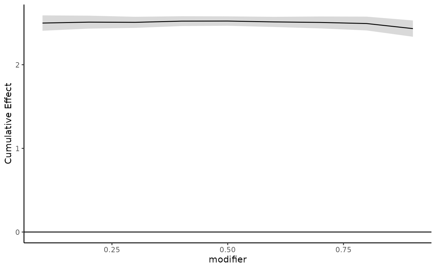
There are two ways to look at estimated point-wise effects: by
modifier or by time. To create a grid of estimated point-wise effect
plots for a select number of time points, specify
plot_by = time and provide select time points to
time_pts. The following plots estimated point-wise effects
across a grid of modifiers isolated for weeks 10, 20, and 30:
plot_DLF(new_modifiers = seq(0.1,0.9,0.1),
         mod_fit = dlim_fit,
         mod_name = "modifier",
         plot_by = "time",
         time_pts = c(10,20,30))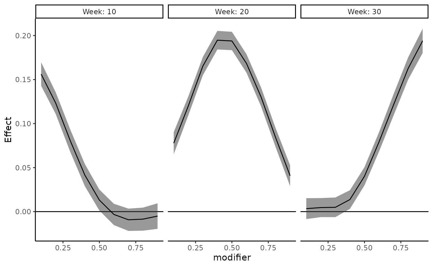
To create a grid of estimated point-wise effect plots for a select
number of modifier values, specify plot_by = modifier and
provide select modifier values to new_modifiers. The
following plots estimated point-wise effects across all time points
isolated for modifier values 0.25, 0.5, and 0.75.
plot_DLF(new_modifiers = c(0.25, 0.5, 0.75),
         mod_fit = dlim_fit,
         mod_name = "modifier",
         plot_by = "modifier")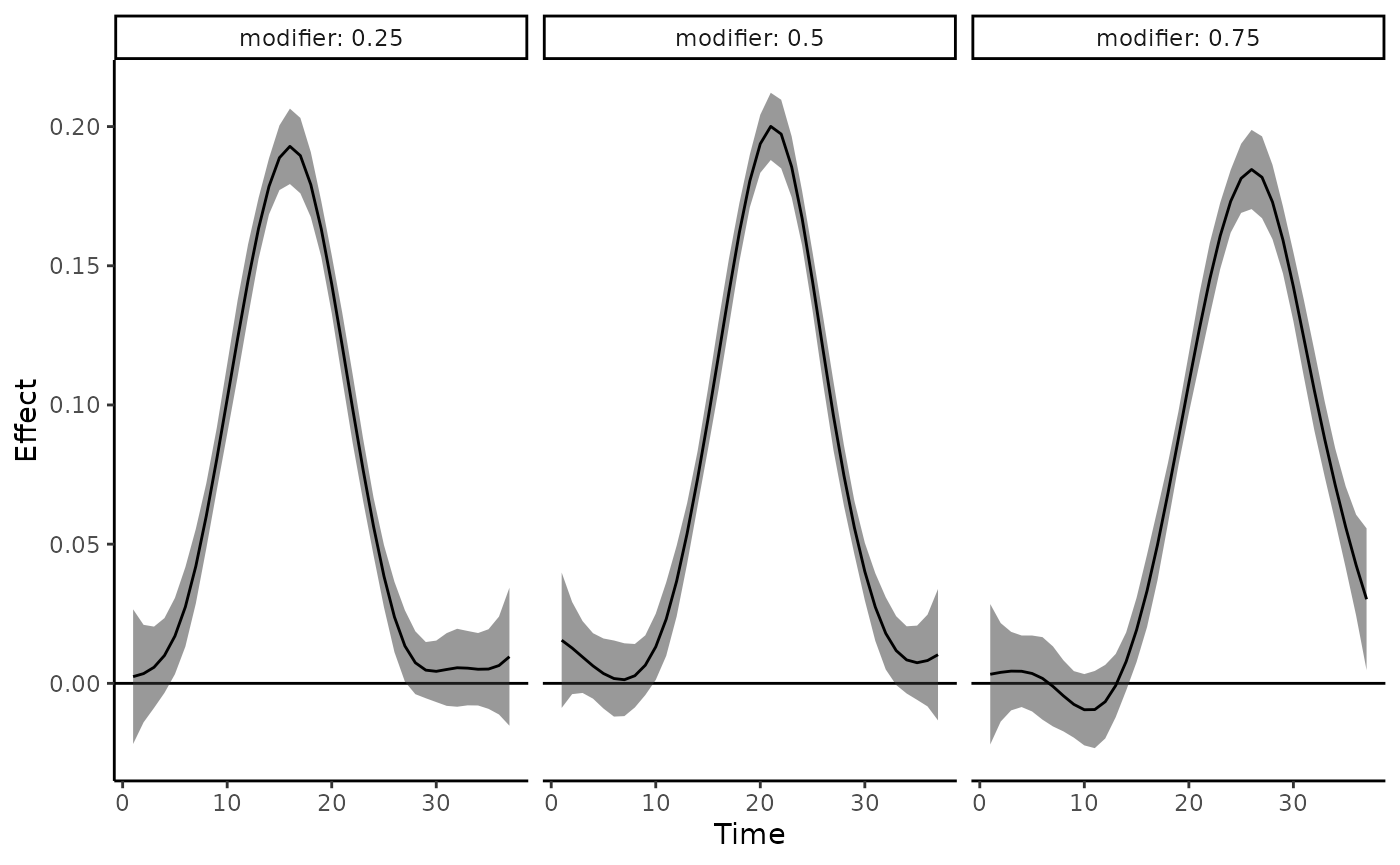
When plotting by point-wise effect estimates, you also have the
option to specify the exposure-time values. If the 37 time points in
this example actually correspond to exposure during months 10 to 46
after parturition and you want to look at the exposure-time-response
functions at months 20, 30, and 40, pass
exposure_time = 10:46 to specify that the 37 time points in
the data correspond to months 10 to 46, and pass
time_pts = c(20,30,40) to specify plotting cross-sections
at months 20, 30 and 40.
plot_DLF(new_modifiers = seq(0.1,0.9,0.1),
mod_fit = dlim_fit,
mod_name = "modifier",
plot_by = "time",
exposure_time = 10:46,
time_pts = c(20, 30, 40))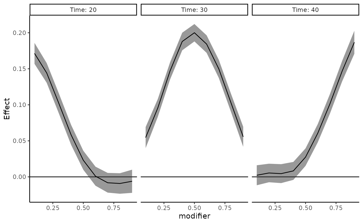 When you pass
 exposure_time = 10:46 to along with
plot_by = "modifier", then plot_DLF plots the
point-wise effects at cross-sections of the new_modifiers
modifier values with appropriately labeled exposure times on the
x-axis.
plot_DLF(new_modifiers = c(0.25, 0.5, 0.75),
         mod_fit = dlim_fit,
         mod_name = "modifier",
         plot_by = "modifier",
         exposure_time = 10:46) +
  xlab("months after parturition")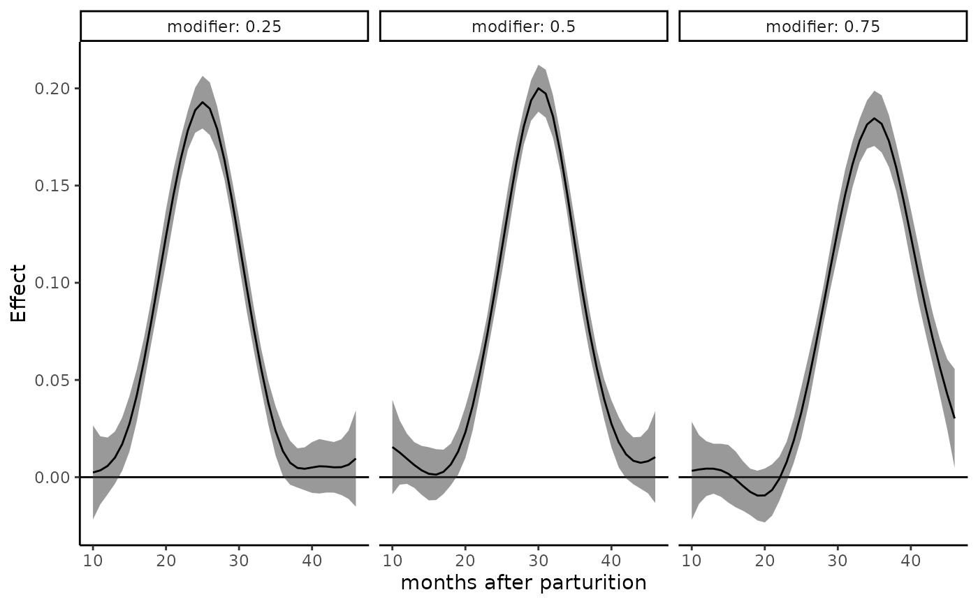
Custom plotting examples
You can use the output from the predict function to
create your own custom plots. To create a custom cumulative effect plot,
specify a range of modifier value through newdata in the
predict function, and then extract the cumulative effect
estimates (dlim_pred$est_dlim$betas_cumul), and the upper
(dlim_pred$est_dlim$cumul_UB) and lower
dlim_pred$est_dlim$cumul_LB bounds for the cumulative
effects. Combine these along with the modifiers into a data frame and
plot using ggplot or plot.
#predict
dlim_pred <- predict(dlim_fit,
                     newdata = seq(0.1, 0.9, 0.1))
#> Returning fitted values is in progress.

#create data frame for plotting
dlim_cumul_df <- data.frame(Estimate = c(dlim_pred$est_dlim$betas_cumul),
                            LB = c(dlim_pred$est_dlim$cumul_LB),
                            UB = c(dlim_pred$est_dlim$cumul_UB),
                            Modifier = c(dlim_pred$est_dlim$modifiers))

#plotting
ggplot(dlim_cumul_df, aes(x = Modifier, y = Estimate)) +
    geom_point(color = "blue") +
    geom_errorbar(aes(ymin=LB, ymax=UB)) +
    geom_hline(yintercept = 0,  color = "black", size=1) +
    xlab("Modifier") +
    ylab("Change in response per unit of exposure") +
    ggtitle("Cumulative Effect Esimates") +
    theme_bw()
#> Warning: Using `size` aesthetic for lines was deprecated in ggplot2 3.4.0.
#> ℹ Please use `linewidth` instead.
#> This warning is displayed once every 8 hours.
#> Call `lifecycle::last_lifecycle_warnings()` to see where this warning was
#> generated.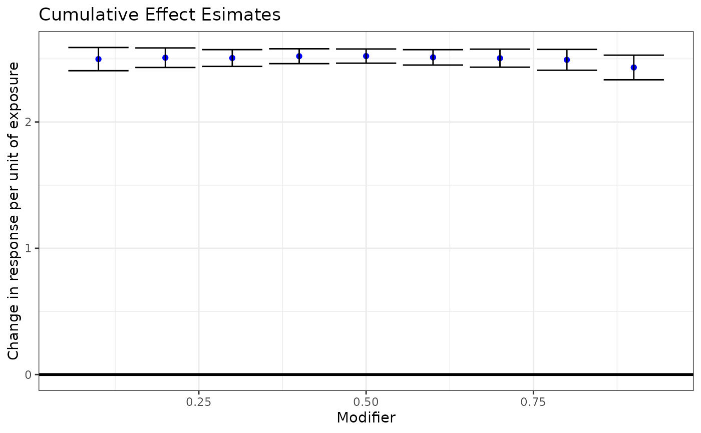
To make a custom plot of the exposure-time-response functions for
specific modifier values, you can follow a similar approach. Specify the
modifiers you want to use with newdata in the
predict function and set type = "DLF" to
obtain point-wise effect estimates. Then extract the point-wise effect
estimates (dlim_pred$est_dlim$betas), and the upper
(dlim_pred$est_dlim$UB) and lower
(dlim_pred$est_dlim$LB) bounds. Note the use of the
transpose function to make sure they are vectorized in proper order. The
dimensions of each of these matrices is the number of modifier values
specified by the number of exposure-time points.
#predict
new_mods <- c(0.25, 0.5, 0.75)
dlim_pred <- predict(dlim_fit,
                     newdata = c(0.25, 0.5, 0.75),
                     type = "DLF")

#create data frame for plotting
dlim_pred_df <- data.frame(Estimate = c(t(dlim_pred$est_dlim$betas)),
                           LB = c(t(dlim_pred$est_dlim$LB)),
                           UB = c(t(dlim_pred$est_dlim$UB)),
                           Week = rep(1:37,length(new_mods)),
                           Modifier = rep(new_mods, each = 37))

#plotting
ggplot(dlim_pred_df, aes(x = Week, y = Estimate)) +
    geom_point(color = "blue") +
    geom_errorbar(aes(ymin=LB, ymax=UB)) +
    geom_hline(yintercept = 0,  color = "black", size=1) +
    facet_grid(cols = vars(Modifier), labeller = "label_both") +
    xlab("Exposure week") +
    ylab("Change in response per unit of exposure") +
    theme_bw()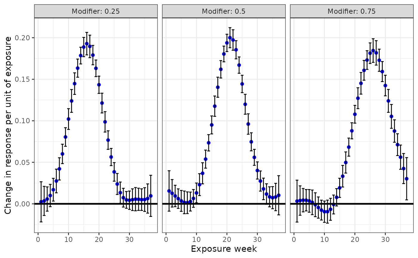
Model Comparison
We can compare this model to a standard DLM using the
model_comparison function. The full model is the
dlim_fit model object, and the null model by default is
"none", a DLM with no interaction (standard DLM). Then,
specify the exposure used to create dlim_fit and the number
of bootstrap samples, B = 5 (we recommend using at least
1000 bootstrap samples, but use 5 to illustrate quickly). The function
returns the decision to reject or fail to reject the null model based on
the default confidence level conf.level of 0.95 along with
an attribute containing the empirical bootstrap p-value.
model_comparison(fit = dlim_fit,
                 null = "none",
                 x = exposure,
                 B = 5)
#>      95%
#> "reject"
#> attr(,"pval")
#> [1] 0
There are 6 different types of model comparisons this function supports:
DLIM with non-linear interaction v. DLIM with quadratic interaction (
attr(fit, "model_type") == "nonlinear"andnull = "quadratic")DLIM with non-linear interaction v. DLIM with linear interaction (
attr(fit, "model_type") == "nonlinear"andnull = "linear")DLIM with non-linear interaction v. standard DLM without interaction (
attr(fit, "model_type") == "nonlinear"andnull = "none")DLIM with quadratic interaction v. DLIM with linear interaction (
attr(fit, "model_type") == "quadratic"andnull = "linear")DLIM with quadratic interaction v. standard DLM without interaction (
attr(fit, "model_type") == "quadratic"andnull = "none")DLIM with linear interaction v. standard DLM without interaction (
attr(fit, "model_type") == "linear"andnull = "none")
Bibliography
Demateis, D., Keller, K. P., Rojas-Rueda, D., Kioumourtzoglou, M.-A., & Wilson, A. (2024). Penalized distributed lag interaction model: Air pollution, birth weight, and neighborhood vulnerability. Environmetrics, e2843. https://doi.org/10.1002/env.2843 >>>>>>> dev